
Trees Are Kernels — and the Kernel Knows Where the Model Is Weak

Chapter 4 of The Learned Kernel. Last time we said the geometry should be learned, not chosen, and named boosting as the first engine that does it. This time we take the kernel a boosted ensemble grows for free and use it for something the black box never offered: a map of exactly where the model fails.
You train an XGBoost model on California housing. It is good. Cross-validated, tuned, an out-of-sample R² of about 0.85. You would ship it.
And you would be shipping a model that is 0.85 on average — a number that quietly averages over the places it is excellent and the places it is not. “On average” is where model risk hides. The question that should keep you up is not how good is it? but where is it bad, and who lives there?
Here is the pleasant surprise of this chapter: the ensemble you just trained already carries the instrument you need to answer that. Its kernel.
The kernel boosting already grew
A decision tree splits the input space into leaves and gives every point in a leaf the same prediction. It never wrote down a notion of “similar,” but it implied one: two points are interchangeable to the tree exactly when they land in the same leaf. Run an ensemble of T trees and you can grade that similarity — count the fraction of trees that route two points to the same leaf.
Write ℓ_t(x) for the leaf that point x reaches in tree t. The leaf kernel is
k(x, x’) = (1/T) Σ_t₌₁ᵀ 1{ℓ_t(x) = ℓ_t(x’)}
Three things are true the moment you write it down. It is an inner product of the one-hot leaf indicators, so it is a genuine positive-semidefinite kernel — slot-in-ready for any kernel method. Its diagonal is 1 (a point shares every leaf with itself). And its values live in [0, 1] — a fraction of trees. Nobody designed it. Boosting did, by fitting the splits to the labels. It is a supervised similarity: two houses are close not because they sit near each other in raw feature space, but because the model learned to treat them the same way for the target.
You could predict with this kernel and recover the ensemble exactly — that was the previous framing, and it is a clean result. But prediction is not the sharpest thing the kernel is good for. The sharpest thing is that it hands you the model’s own map of the data, and on that map you can see the weak spots.
We won’t predict with it — we’ll navigate by it
The kernel is an n × n object: how similar is every training point to every other? For 16,512 houses that is 273 million numbers, and the honest way to find its structure — a spectral embedding, the eigenvectors of the normalized kernel — costs O(n³). That is the wall this series keeps running into.
Nyström (we are going to cover this in the future) is the way through. Pick a modest set of m landmark points, build the eigenbasis on the small m × m block, and extend it to all n points through their kernel similarity to the landmarks. The eigensolve is bounded by m, and everything else is O(n·m) — linear in the data. On a laptop this turns “spectral clustering is intractable” into “spectral clustering finished before your coffee.” No subsampling of your data; the whole training set flows through, only the internal support is capped.
Cluster the points in that spectral embedding and you get regions the model’s geometry treats as coherent — groups of houses the ensemble routes through the same leaves, for the same reasons. Not regions you drew with a lat/long box. Regions the model itself believes in.
In Modeva (download for free: https://modeva.ai/) this is one call. Build the leaf kernel by restricting a FuseKernel to its XGBoost channel — no RBF, no learned spectral component, just the pure leaf co-membership — and ask it to break itself down:
fk = MoFuseKernelRegressor(backend="xgboost",
                           use_xgb=True, use_rbf=False, use_spectral=False,
                           solver="nystrom", gbdt_params=best_params)
fk.fit(ds.train_x, ds.train_y.ravel())

weak = fk.diagnose_weak_clusters(ds, n_clusters=5)   # Nyström spectral clustering
weak.table                                           # performance, per cluster
The weakness map
diagnose_weak_clusters does the Nyström spectral clustering, then reports the model’s metric inside each cluster, on train and test. Here is what “0.85 on average” was hiding:
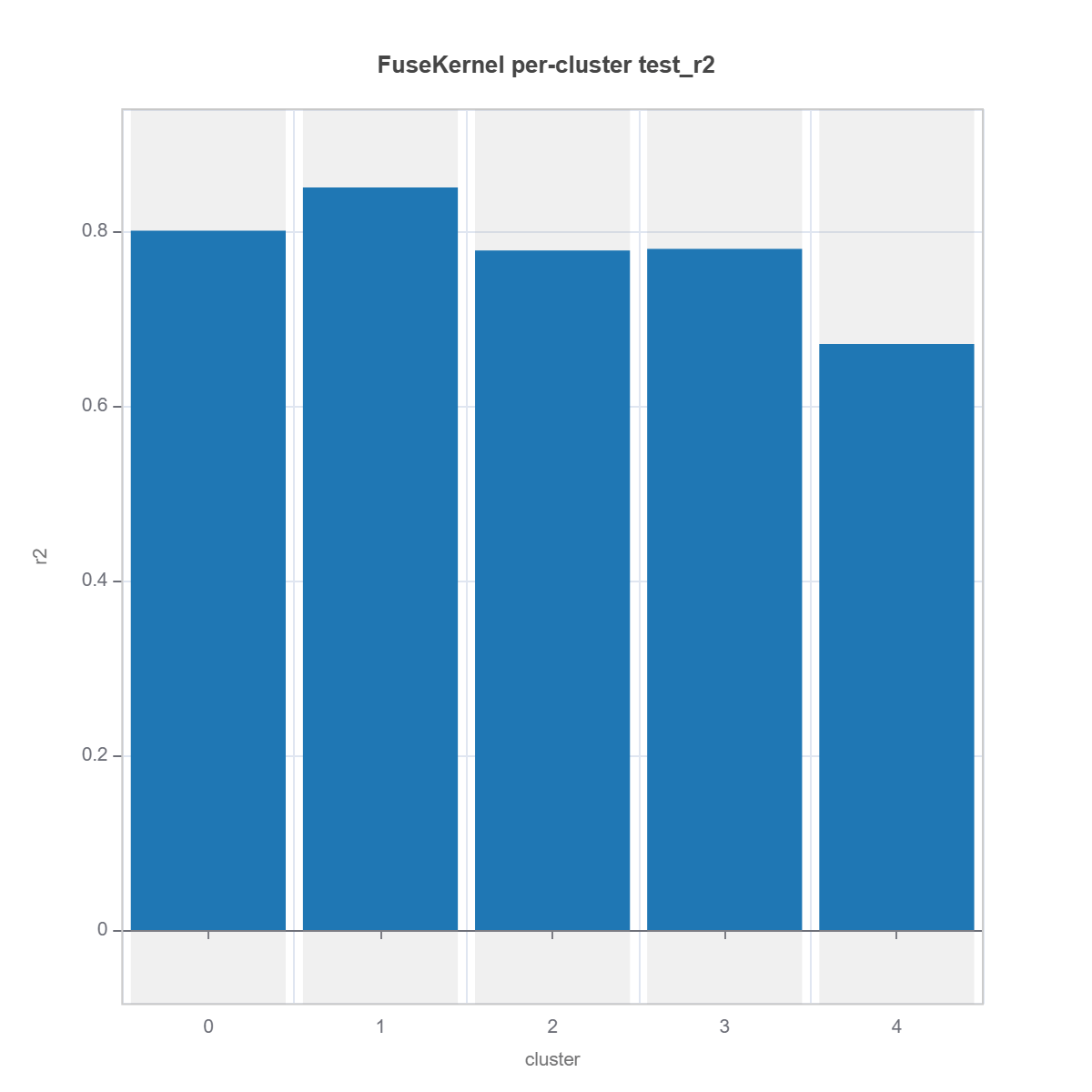
The full test set scores R² ≈ 0.85. But cluster by cluster, the model ranges from 0.85 in its best region down to 0.67 in its worst — a fifth of the data where a quarter of the explained variance simply evaporates. Same model, same day, same metric. The average was telling the truth and hiding it at the same time.
This is the move that matters. We did not go hunting for the weak region with a feature we suspected. We let the model’s own kernel partition the data, and the partition surfaced a region where the model is materially worse. The geometry boosting learned for accuracy doubles as a geometry for diagnosis.
Where, exactly — and who lives there
A weak cluster is only actionable if you can say where it sits. So take the weakest cluster, set it against the rest of the data, and ask — feature by feature — how differently it is distributed. The tool is the Population Stability Index, the same PSI https://modeva.ai/docs/2-user-guide/testing/resiliencerisk teams already use to watch for drift; here we point it inward, at one cluster versus its complement.
That is, again, a shipped test — the identical data_info → data_drift_test pattern the resilience diagnostic uses. Build the weak-vs-rest split from the cluster labels the diagnosis already returned, and run it:
labels   = np.asarray(weak.value["labels_train"])
worst_id = int(weak.value["worst_clusters"].iloc[0]["cluster"])
drift = ds.data_drift_test(
    dataset1="train", sample_idx1=np.where(labels == worst_id)[0],
    dataset2="train", sample_idx2=np.where(labels != worst_id)[0],
    distance_metric="PSI")
drift.plot("summary")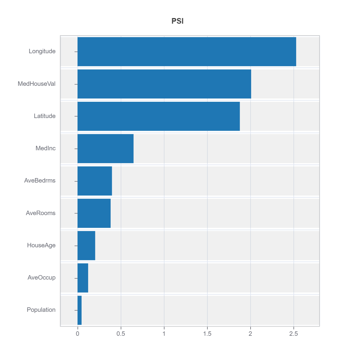
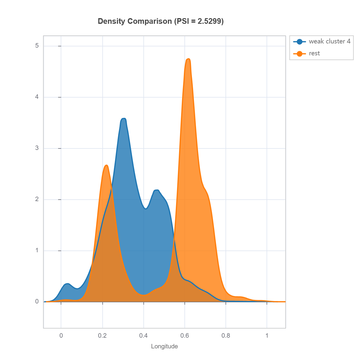
The ranking is unambiguous. Longitude (PSI 2.53), median house value (2.01), and latitude (1.88) tower over everything else — all far past the 0.25 “large shift” line, while the remaining features barely move. The weak region is not spread thinly across the state. It is a geographic pocket — a specific band of longitude and latitude — where prices are distributed unlike anywhere else, and where the ensemble’s leaf geometry, however good on average, does not carve finely enough.
Overlay the density of the top-PSI feature, weak cluster against the rest, and the shift is not a statistic anymore — it is a picture:
What you do with a weak region
Knowing where changes what you can do. You can flag it — the honest move — and tell downstream users the model’s confidence is thinner in that band. You can go get more data there. Or you can repair it in place: fit a specialist that only has to be good in the weak geometry and let a gate route to it — a mixture of experts, or a residual correction fit out-of-fold in the very same leaf kernel. That repair is the next chapter.
But the principle is already the point. A model trained purely for accuracy carries, for free, a supervised map of its own competence. You do not have to guess where it is weak, or probe it feature by feature hoping to trip over the failure. You ask the kernel the model already grew, and it shows you — with a spectral embedding to find the regions and a PSI to name them. Discover where the model fails; don’t declare where you think it might.
Run it yourself
Everything above is a handful of calls in Modeva — data loading, the cross-validated XGBoost, the leaf kernel, the Nyström clustering, and the PSI drift test are all first-class. It is free to use: generate a licence and install in one line at modeva.ai.
# pip install modeva  (get your free licence key at https://modeva.ai/)
from modeva import DataSet, TestSuite
from modeva.models import MoXGBRegressor, MoFuseKernelRegressor, ModelTuneGridSearch

ds = DataSet(); ds.load(name="CaliforniaHousing")
ds.set_random_split(test_ratio=0.2, random_state=0)
ds.scale_numerical(features=(ds.target_feature_name,), method="log1p")  # skewed target
ds.preprocess()

# cross-validate, then keep the BEST setting (lowest CV MSE)
hpo = ModelTuneGridSearch(dataset=ds, model=MoXGBRegressor(max_depth=3))
cv  = hpo.run(param_grid={"n_estimators": [100, 200, 300],
                          "learning_rate": [0.03, 0.05, 0.1]},
              metric=("MSE", "MAE", "R2"), cv=5)
best_params = cv.value["params"][cv.table["MSE"].idxmin()]
The companion notebook runs top to bottom on the full dataset — tune, build the leaf kernel, cluster it with Nyström, draw the per-cluster performance bar, and rank the weak region by PSI with a density overlay.
▶ Run it in Colab (no install): open in Colab
📦 Code: https://github.com/asudjianto-xml/MRM/tree/main/Tabular
🔑 Get Modeva (free): https://modeva.ai/
The previous installment, From Chosen to Learned Kernels, is where the discipline behind these supervised kernels — and the leakage they invite — comes from.
Your gradient-boosted ensemble is a kernel machine, and its kernel is a supervised map of the data. Read the map with a Nyström spectral embedding and it partitions the model into regions of competence; score each region and the weak spots surface on their own; name them with PSI and you know exactly which slice of the world to worry about. Next week: repairing the weak region without touching the parts that already work.
The Learned Kernel is a free weekly series. The posts carry the intuition and the runnable code; every example runs on Modeva — modeva.ai.