
TransE: Translation as a Decoder

This is the second post in Knowledge Graphs as Geometry, a weekly series that builds one idea, chapter by chapter: a knowledge graph stores facts as relations, every relation is an operation in space, and predicting a missing fact is geometry. Last week we made the case that a relation is an operation and a score is a distance. This week we build the very first model that runs on that idea — the simplest operation there is, a translation — and we watch exactly where it breaks. The break is not a bug. It is a fact of geometry, and calling it is what forces every richer model in the rest of the series.
Start with the family from last week (https://agussudjianto.substack.com/p/a-relation-is-an-operation). Ann and Bob are married and have two children, Carol and Dave. Carol married Eve, and they have a child, Frank. Now pick the simplest possible way to turn the relation parentOf into an operation in space: make it a single arrow, a fixed step you take from any parent to land on their child. Add that one arrow to Ann and you should land on her child. Add it to Carol and you should land on Frank.
That is the whole idea behind TransE, the model that launched modern knowledge graph embeddings. A relation is a displacement — one vector you add to the head to predict the tail. It is the cleanest instance of the reframe from last week, and because it is so clean we can train it, see it work, and put our finger on the precise thing it cannot do. The thing it cannot do is the reason the book has thirteen more chapters.
A relation is a displacement
Give every entity a vector in ℝᵈ, a position we get to learn. Give every relation a vector too. TransE asks a true triple (h, r, t) to satisfy
The relation vector 𝐫 is the displacement that carries the head to the tail. To turn that “≈” into a number we can rank, we measure how close the translated head lands to the actual tail and negate it, so that closer means higher:
Here γ is just a margin, a constant that shifts every score to a convenient operating point; it does not change any ranking. This is the prototype of what the book calls a distance decoder: build a relation-conditioned prediction 𝐭̂ = 𝐡 + 𝐫, then score a candidate tail by how far it sits from that prediction. In the language of the series, the operation Fᵣ is the simplest map there is — Fᵣ(𝐡) = 𝐡 + 𝐫 — and the comparator is Euclidean distance.
Every model in this series answers the same three questions, and TransE is where we ask them for the first time. What is the carrier — the thing an entity is? Here it is a vector in ℝᵈ. What is the operator — the map a relation applies to it? Here Fᵣ(𝐱) = 𝐱 + 𝐫. And what is the comparator — the rule that turns a prediction and a candidate into a score? Here the negated distance. Hold those three slots in mind, because the entire book is the story of leaving the carrier and comparator alone and making the operator richer.
That last point deserves a name now, because we will lean on it for thirteen more chapters. Every operator in the book is one affine map,
where the linear part Mᵣ factors as Mᵣ = Uᵣ Σᵣ Vᵣᵀ — a rotation, an anisotropic stretch, another rotation — and 𝐜ᵣ is a translation. TransE is the simplest possible setting of that dial: Mᵣ = I and 𝐜ᵣ = 𝐫. The linear part is the identity, so the operator does nothing but slide. Every richer model we meet later — bilinear, rotational, the full Clifford machine — turns Mᵣ away from the identity. Seen that way, TransE is not a different kind of model from the rest of the book; it is the rest of the book with the matrix switched off.
The picture is literal. Learning parentOf means finding one vector 𝐫 that, added to a parent, lands near the child. Added to Ann it should reach Carol; added to Carol it should reach Frank. One arrow, reused for every parent in the graph. That reuse is exactly why the model can generalize to a parent edge it never saw — and, as we are about to find out, exactly why it strains against relations that are not so simple.
Training when you only have positive facts
A knowledge graph stores facts that are true. It does not store a curated list of falsehoods, which means there are no negative examples to train against. TransE manufactures them. For each true triple (h, r, t) it corrupts the head or the tail with a random entity to make a negative (h′, r, t′), then uses a logistic loss that pushes the true triple’s score up and the corrupted ones down:
The weights wᵢ are uniform for ordinary negative sampling, or self-adversarial — larger for the negatives the model currently scores highly — which spends the training budget on the hard, near-miss negatives instead of the obvious ones. A negative that swaps a person for an unrelated concept is already scored far away and teaches the model almost nothing; a negative that swaps the true child for a plausible one is right at the decision boundary, and that is where the gradient should go. Self-adversarial weighting is just the bookkeeping that puts it there.
One more ingredient matters: before each use, entity vectors are renormalized to the unit sphere, ‖𝐞‖ = 1. That is the regularization the original model leans on in place of weight decay, and it stops the embeddings from drifting off to infinity to make distances trivially large. Without it, the cheapest way to lower the loss is to push every entity far apart so that even a sloppy displacement looks accurate; the constraint takes that escape away. Keep the unit-sphere idea in mind, because it is what makes the failure we are about to see so vivid: every entity lives on the same circle, so when two of them have to occupy the same spot, they have nowhere to hide.
Put together, one training step is short. Sample a batch of true triples. Corrupt heads or tails to manufacture negatives. Renormalize the entity vectors back onto the sphere. Score everything with γ − ‖𝐡 + 𝐫 − 𝐭‖, form the logistic loss above, and take a gradient step. Repeat. There is no curated negative set, no special machinery — the whole method is “predict the tail by sliding, and learn the slide from contrast.”
The whole loop lives in the library. In kge, kge.models.TransE carries the score and the unit-norm constraint, and kge.train.Trainer runs the loss above with either weighting. The chapter notebook just configures it.
Demonstration 1: watch the displacement, and watch the collapse
Train TransE on the twelve family triples with a two-dimensional embedding — small enough that we can plot every entity on the page — and draw the learned parentOf displacement as an arrow from Ann. The arrow’s tip is where the model predicts Ann’s child should be.
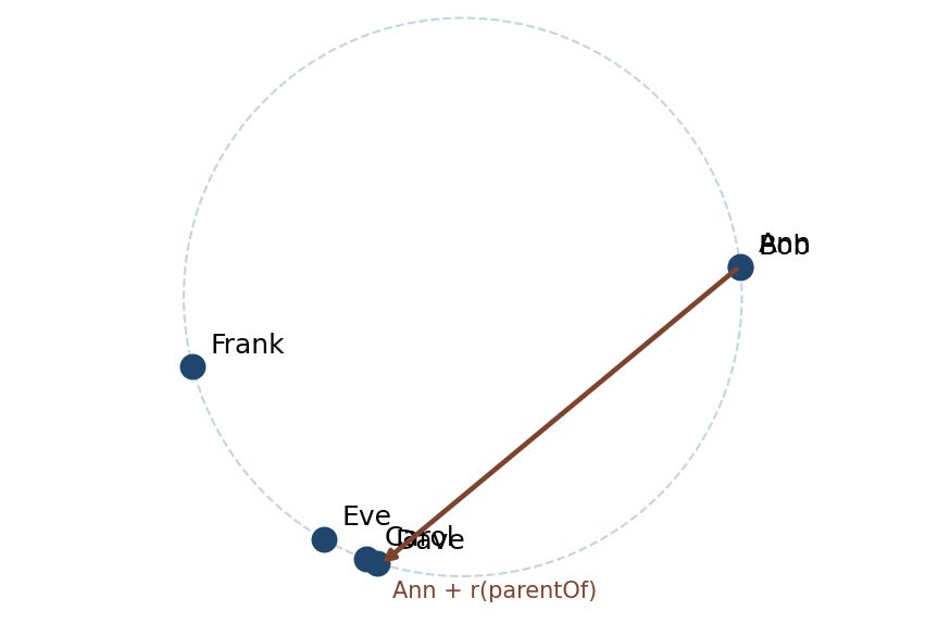
TransE on family graph (dimensionality = 2): the collapse
Look at where the entities landed. The arrow from Ann points down to a single spot near the bottom of the circle — and Carol and Dave are sitting on top of each other at that spot, two labels printed over one point. Up at the top right, Ann and Bob have merged the same way, two labels on one point. This is not a plotting glitch and it is not undertraining. It is the model solving an impossible request in the only way it can.
Here is the request. Ann is a parent of both Carol and Dave, so the single arrow 𝐫 added to Ann has to land near Carol and near Dave at the same time. There is only one way one arrow can reach two targets: make the two targets the same point. So training pulls Carol and Dave together. Likewise Carol has two parents, Ann and Bob, and the only way 𝐡 + 𝐫 can reach Carol from both is to pull Ann and Bob together. The model fits the graph by destroying the distinctions it was supposed to keep.
You might suspect this is an artifact of squeezing the graph into two dimensions, and that more room would fix it. It would not. The conflict is between a single fixed arrow and a relation that wants to fan out, and adding dimensions does not change the arithmetic 𝐡 + 𝐫 = one point. Higher dimensions give the optimizer more directions to spread unrelated entities apart, which is why the collapse is so stark on a tiny graph and only somewhat softened on a large one — but the co-answers of a many-valued relation still have to converge, in any dimension, because the constraint is the same. We use two dimensions here only because it lets us see on a page what the metrics will later only let us infer.
Demonstration 2: the residuals lie, the distances tell the truth
The seductive thing is that, if you only check the training loss, TransE looks like it nailed parentOf. Measure the residual — how far 𝐡 + 𝐫 lands from each true child — and both are essentially zero.
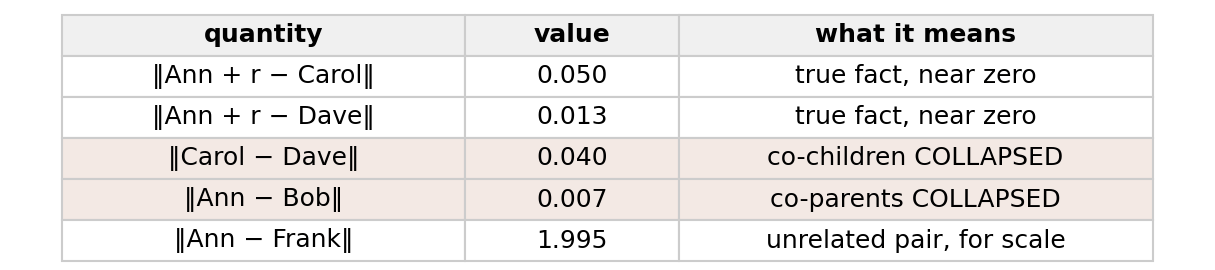
Both residuals are tiny but only because the anser collapsed.
Read the first two rows: ‖Ann + 𝐫 − Carol‖ ≈ 0.05 and ‖Ann + 𝐫 − Dave‖ ≈ 0.01. The translated head lands on both children, just as the model was asked. If you stopped here you would conclude TransE represents parentOf perfectly. It does not, and the next two rows say why. ‖Carol − Dave‖ ≈ 0.04 and ‖Ann − Bob‖ ≈ 0.007: the co-children and the co-parents are now the same point, while an unrelated pair like Ann and Frank sits a full ‖·‖ ≈ 2 apart — the diameter of the unit circle. The residual is small only because the answers are no longer distinct.
This is the heart of the chapter. The two facts of translation that cause it are not training artifacts; they are geometry, and each is a one-line argument. A translation Fᵣ(𝐱) = 𝐱 + 𝐫 is single-valued — it is a function, so 𝐡 + 𝐫 names exactly one point, which means it cannot place one head near several distinct tails at once. And it is injective — if 𝐡₁ + 𝐫 = 𝐡₂ + 𝐫, subtract 𝐫 from both sides and 𝐡₁ = 𝐡₂, so it cannot send several distinct heads to one tail. Neither fact mentions training, the loss, or the optimizer. They are properties of addition.
Now read them against parentOf. Ann is a parent of both Carol and Dave: a single arrow added to Ann must reach two distinct targets, which single-valuedness forbids unless the targets coincide. Carol has two parents, Ann and Bob: two distinct heads plus the same arrow must reach Carol, which injectivity forbids unless the heads coincide. A many-to-many relation trips both wires. No amount of training escapes the proposition; the optimizer can only pay the price the geometry demands, and the price is collapsed entities. What the figure shows is not a model that trained badly. It is a model that trained perfectly against an impossible constraint and paid in the only currency it had.
Demonstration 3: symmetry forces the relation to vanish
There is a second rigidity, and it bites a different family of relations. Look at spouse. If Ann is married to Bob then Bob is married to Ann — the relation is its own reverse. Write what translation needs for that: from the first fact, Bob = Ann + 𝐫; from the second, Ann = Bob + 𝐫. Substitute and you get 𝐫 = −𝐫, which forces 𝐫 = 𝟎. A symmetric relation can only be a translation if the translation is nothing. And a zero displacement makes 𝐡 + 𝐫 = 𝐡, so the model predicts every entity is its own spouse.
The trained model shows exactly this. Read off the learned displacement norm for each relation in the family graph.
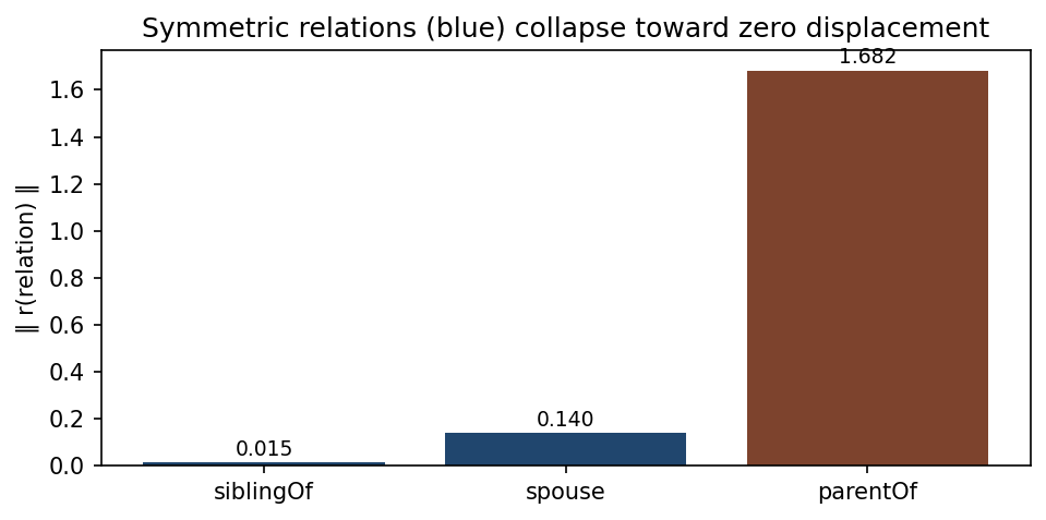
The two symmetric relations, spouse and siblingOf, carry the smallest displacements by far — ‖𝐫‖ ≈ 0.14 and ≈ 0.015, both pinned toward zero — while the directed parentOf carries a real arrow at ‖𝐫‖ ≈ 1.68. Training drove the symmetric relations toward the only translation that can be symmetric, which is no translation at all. The geometry told us in advance: symmetry is a half-turn, and a half-turn is a rotation, and TransE has no rotations. It has one tool, addition, and addition cannot turn around.
So we already see the two patterns from last week’s table showing up as hard limits. Cardinality (many-to-many) forces a collapse. Symmetry forces a vanishing. Both come straight from the choice to make Fᵣ a translation, and both are the reason the rest of the series reaches for richer operations.
Demonstration 4: the fingerprint at scale
None of this makes TransE useless. It makes its errors structured and recognizable, and that is more interesting. The structure shows up as a signature in the accuracy numbers — a fingerprint you can read off the metrics without ever looking at the embeddings.
Train TransE for real on UMLS, a small medical knowledge graph (135 entities, 46 relations) that fits in seconds on a laptop, and grade it with the filtered ranking protocol from last week. Then put it next to TransE on WN18RR, a 40,000-entity WordNet graph trained on a GPU, whose numbers we carry as a cached result rather than retraining live.
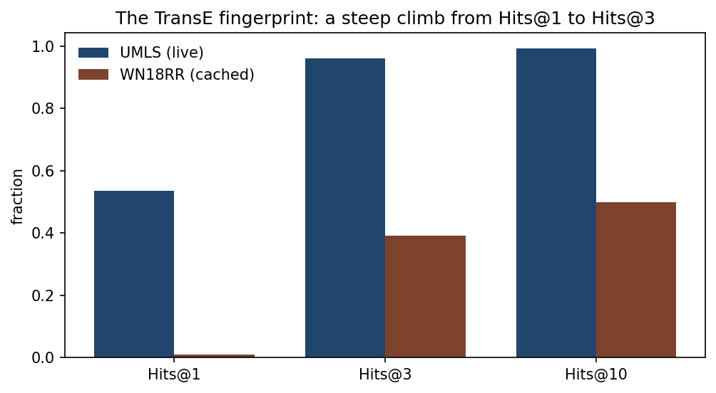
Look at the shape, not the height. On UMLS the model gets the right answer into the top three almost always — Hits@3 ≈ 0.96 — but lands it at rank one only about half the time, Hits@1 ≈ 0.53. On WN18RR the same shape is dramatic: the model reaches a filtered MRR of 0.213, with Hits@3 ≈ 0.39 but Hits@1 ≈ 0.01 — barely one query in a hundred resolved exactly. In both cases the climb from Hits@1 to Hits@3 is steep. TransE reliably finds the right neighborhood and reliably fails to pick the one right answer out of it.
That steep climb is the collapse from the family graph, scaled up. When parentOf forced Carol and Dave onto the same point, the model could land near the cluster but could not separate the members. On a big graph full of symmetric and many-valued relations the same thing happens everywhere: the true tail sits in a tight clump of co-answers the single displacement squashed together, so it shows up near the top — but rank one is a coin flip among the clump. WN18RR is full of exactly these relations — hypernym and synonym chains, symmetric “see also” and “derivationally related” links — which is why its fingerprint is the extreme case, a Hits@3 near 0.39 over a Hits@1 near 0.01. UMLS is milder because more of its relations are close to single-valued, so the clumps are smaller and rank one is reachable more often. Same mechanism, two doses.
There is a useful discipline hiding here. We never had to open the embeddings to diagnose the problem. The metric profile alone — a wide gap between Hits@1 and Hits@3 — is enough to say “this model is landing the neighborhood and missing the point,” which is the signature of rigidity. The fingerprint is the rigidity proposition made visible in a number you already compute. When we meet ComplEx in the next chapter we will see the opposite fingerprint — a high Hits@1, the gap closed — and read it as the signature of a model that turned the matrix Mᵣ back on and escaped exactly this rigidity.
Run it yourself
The core is a handful of lines: build the graph, train TransE, then measure the collapse directly.
from kge.data import TripleFactory
from kge.models import TransE
from kge.train import Trainer, TrainConfig
import torch, torch.nn.functional as F

triples = [("Ann","parentOf","Carol"), ("Bob","parentOf","Carol"),
           ("Ann","parentOf","Dave"),  ("Bob","parentOf","Dave"),
           ("Ann","spouse","Bob"),     ("Bob","spouse","Ann")]
g = TripleFactory(train=triples, valid=[], test=[], name="family")

model = TransE(g.n_entities, g.n_relations, dim=2, margin=2.0, p_norm=2)
Trainer(model, g, TrainConfig(mode="1vsall", epochs=400, lr=0.05), device="cpu").fit()

E = F.normalize(model.entity.weight, dim=-1)
gap = (E[g.ent2id["Carol"]] - E[g.ent2id["Dave"]]).norm()
print(f"||Carol - Dave|| = {gap:.3f}")   # ~0.04: collapsed to fit (Ann,parentOf,*)
The companion notebook trains TransE on the family graph, plots the displacement and the collapse, measures the residuals and the relation-norm vanishing, and then reproduces the Hits@1-versus-Hits@3 fingerprint live on UMLS with the WN18RR number alongside — every figure in this post, executed.
▶ Run the notebook in Colab: https://colab.research.google.com/github/asudjianto-xml/Knowledge-Graph-Geometry/blob/main/notebooks/ch02_transe.ipynb
Notebook: https://github.com/asudjianto-xml/Knowledge-Graph-Geometry/blob/main/notebooks/ch02_transe.ipynb
📦 Code: github.com/asudjianto-xml/Knowledge-Graph-Geometry — pip install "kge-geometric @ git+https://github.com/asudjianto-xml/Knowledge-Graph-Geometry.git"
TransE makes a relation a single displacement: 𝐡 + 𝐫 ≈ 𝐭, scored by distance. That one choice is its elegance and its cage. A translation is single-valued and injective, so a many-to-many relation can only be fit by collapsing the entities it should keep apart, and a symmetric relation can only be fit by vanishing to the zero displacement. Its fingerprint — the right answer near the top but rarely at it — is that cage made visible. The rest of the series is one long answer to a single question: how do we relax the rigidity of a lone displacement while keeping its geometric clarity? Next week, the first escape — bilinear models, and the leap from a displacement to a matrix.
Knowledge Graphs as Geometry is a free weekly series adapted from my book Knowledge Graph Embeddings as Geometric Operators. The posts carry the intuition and the runnable code; the book carries the full derivations. Subscribe to follow the whole argument — from a single translation to one operator that contains the entire model zoo.