
The Kernel as the Normal Form
Post #2 of The Learned Kernel.

Last time we saw that every model is a weighted vote over training labels, and the weights are a geometry https://agussudjianto.substack.com/p/the-geometry-hidden-in-every-model. This time we collapse five famous methods into one machine — and find that the only thing you ever really choose is that geometry.
Here is a workflow you have probably run. You have a tabular dataset, so you try a support vector machine or gradient boosting machine. Then a Gaussian process, because you want uncertainty. Then kernel ridge regression because it is fast. Maybe a nearest-neighbor baseline. You compare validation scores and pick a winner, and you call this a model search.
It is not a model search. It is a geometry search wearing a disguise. Those methods are not five different ideas about how to predict — they are one machine, run five times with five different settings of two minor knobs. Underneath, each one does the identical thing: fix a notion of similarity between points, form the table of all pairwise similarities, and solve one linear system. The thing that actually changes your answer is the notion of similarity. Everything else is bookkeeping.
This post makes that precise. By the end, the support vector machine, gradient boosting machine, the Gaussian-process posterior mean, kernel ridge regression, Nadaraya–Watson smoothing and a single head of attention will all be the same object, and the question that drives the rest of the series will be unavoidable: if the only real choice is the geometry, why on earth would you fix it by hand?
From weights to a kernel
Last chapter’s prediction was a weighted vote,
and we noticed the weight on training case i is really a similarity, k(x, xᵢ): how much xᵢ counts when we predict at x. To build a machine on it we ask k to satisfy two conditions. It should be symmetric, k(x, x’) = k(x’, x) — if x’ is like x then x is equally like x’. And it should be positive semidefinite: stack the pairwise similarities into the matrix K with Kᵢⱼ = k(xᵢ, xⱼ), and for any weights c,
That matrix K is the Gram matrix, and a symmetric function whose Gram matrix is always PSD is a positive-semidefinite kernel. The two conditions look technical but they buy two concrete things. First, the eigenvalues of K are nonnegative, so K + λI has eigenvalues at least λ and is always invertible — the linear system at the center of the machine never fails to have a unique answer. Second, and this is the deeper fact, PSD is exactly the condition that lets you write k(x, x’) = ⟨φ(x), φ(x’)⟩ for some feature map φ. The kernel is an inner product in some space. It is, abstractly, a geometry — and the only question is which one.
The reproducing property, in one breath
You almost never need to write φ down, and that is the whole trick. The feature space of a kernel is its reproducing-kernel Hilbert space, and it comes with one fact we lean on constantly: evaluating a function at a point is the same as taking an inner product against the kernel slice at that point,
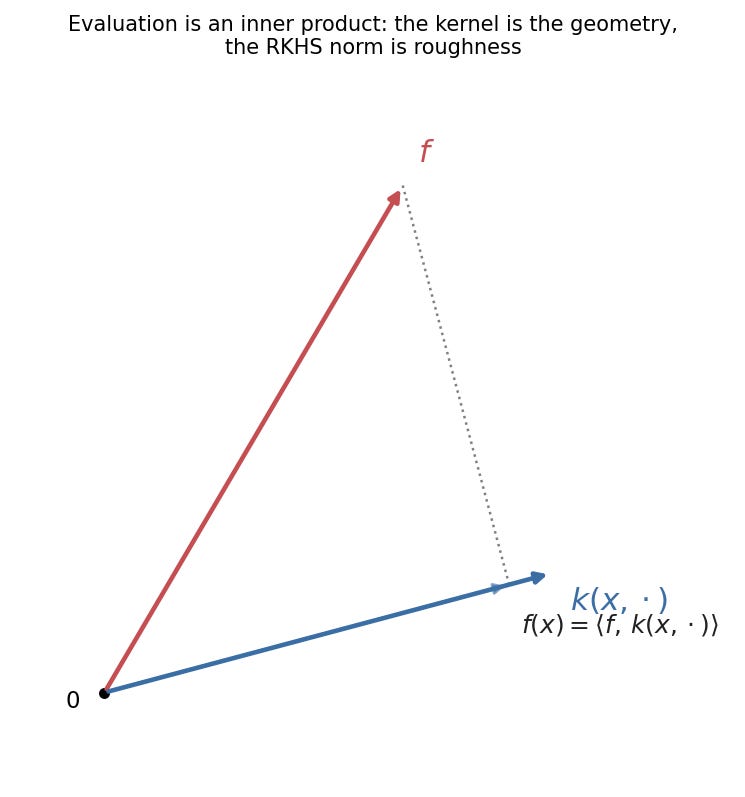
That single equation (pictured above as a projection) is what collapses every method below into one. The space also carries a norm, ‖f‖, and the norm measures roughness in the geometry the kernel defines. Picture two functions that fit the training points equally well. One moves gently, varying only where the kernel says nearby points sit; the other spikes up and down between points the kernel considers far apart. The second has the larger norm — the kernel charges it for disagreeing with the geometry. So when we regularize a fit by ‖f‖², we are not penalizing size in the abstract. We are penalizing roughness as the kernel measures roughness. The regularizer is the geometry. Change the kernel and you change what counts as a simple function, which is the same as changing what the model will believe before it has seen much data.
One derivation: kernel ridge regression
Write the learning problem as fitting the data without fighting the geometry — squared error plus a roughness penalty:
This is an optimization over a possibly infinite-dimensional space, which sounds impossible. It is not, because of the representer theorem: the best f is always a finite combination of the kernel slices at the training points, f(·) = Σⱼ αⱼ k(xⱼ, ·). The reason is a one-line geometric argument — any part of f orthogonal to those slices changes no training prediction but adds norm, so the optimum throws it away. Substitute the finite form and the problem becomes a linear system in the coefficient vector α, with a closed-form solution:
This is kernel ridge regression. And look what it is: last chapter’s weighted vote, with the weights computed by one solve against the Gram matrix,
The vote is back, derived rather than asserted. Notice two things. The first is that the answer is closed form — no gradient descent, no early stopping, no random seed. You build one matrix and solve one system, and the predictor is determined. Very little in modern machine learning has that property, and it is the kernel machine’s quiet advantage: the fit is a fact about the data and the kernel, not an artifact of how long you trained. The second is the shape (K + λI)⁻¹. Hold onto it — the entire scaling story later in the book is a fight with that one inverse, because forming and inverting an n-by-n matrix is exactly what stops you at a few thousand rows on a laptop.
Four faces of the same machine
Now the payoff. Fix one shared Gaussian kernel — k(x, x’) = exp(−‖x − x’‖²/2ℓ²), bandwidth ℓ set by the usual median-distance heuristic, on the California housing data — and predict the same Los Angeles block from Chapter 1 five different ways.
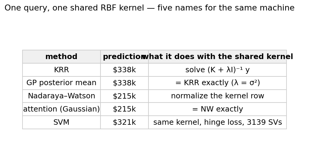
Read the table top to bottom.
The Gaussian process is kernel ridge regression. The GP posterior mean under noise variance σ² is ŷ(x) = k(x,·)ᵀ(K + σ²I)⁻¹y. Set σ² = λ and that is the same formula — not similar, identical. On this block KRR and the GP mean both return $338k, equal to the last decimal. The GP is not a different predictor; it is KRR plus a variance you also get for free. We prove the full posterior in a later chapter, but the best guess is already in hand.
Nadaraya–Watson is the same kernel, normalized instead of solved. Rather than invert K + λI, just make the kernel row sum to one:
This is the case-based face — a literal weighted average of neighbors. It returns $215k here, well below KRR’s $338k, and that gap is the lesson, not an embarrassment. A broad normalized average reaches across a wide neighborhood and gets pulled toward the regional mean; the regularized solve fits the local structure more sharply. Same kernel, different number, because normalizing is not solving. Narrow the bandwidth and the two move toward each other.
Attention is Nadaraya–Watson with a score for a kernel. A single attention head computes Σᵢ softmax(qᵀkᵢ/√d) vᵢ. Read the query q as the test point, the keys kᵢ as training inputs, the values vᵢ as the labels — and this is exactly the normalized smoother above, with the softmax doing the normalizing and exp(qᵀkᵢ/√d) playing the role of the kernel. Give attention a Gaussian score and it is Nadaraya–Watson: on this block it returns the identical $215k. There is one difference in the score real transformers use, and it will matter enormously later: qᵀkᵢ is asymmetric, because queries and keys are projected by different matrices, so its implied kernel need not satisfy k(x, x’) = k(x’, x). We flag that asymmetry now and spend two later chapters earning the right to remove it. For prediction over rows that have no inherent order, it is a liability.
The support vector machine is the same kernel with a different loss. Swap squared error for the hinge loss and you get a kernel machine whose solution is sparse — most coefficients are zero, and the prediction leans only on the “support vectors.” Same Gram matrix inside. Here it returns $321k, close to KRR, using 3,139 of 4,000 points as support vectors. The sparsity is real but dataset-dependent; on a broad kernel, “only the support vectors” can be most of the data.
Put the five side by side and the structure is unmistakable:
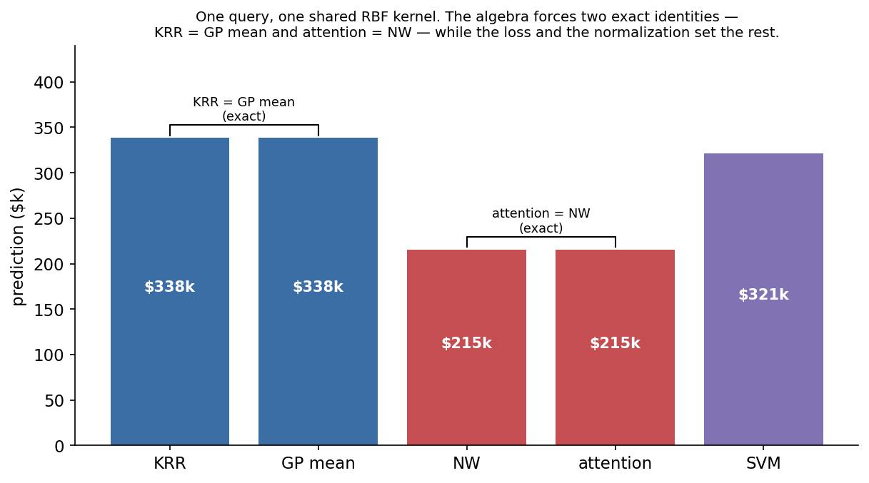
Two pairs are welded together by algebra — KRR equals the GP mean, attention equals Nadaraya–Watson — and the spread between the pairs is set entirely by which loss you picked and whether you normalized. None of it is set by the kernel. The kernel is the one thing all five share.
This reframing earns its keep the moment you stop arguing about methods. A practitioner who has been asking “SVM or GP or boosting?” has been asking a question whose answer barely moves the prediction. The question that moves it — which similarity, at what scale, in which directions — was hiding inside the kernel the whole time, unexamined, usually left at a default. And because the prediction is the weighted vote w(x) = (K + λI)⁻¹k(x,·) regardless of which face you wear, anything you can read off that vote — which training cases carried the prediction, how concentrated the evidence was — transfers across all five. You do not get a separate interpretability story for the SVM and the GP. You get one, attached to the geometry.
Why “normal form” matters
So count the degrees of freedom. Once these five are one machine, the choice of method dissolves into two small decisions — which loss, normalize or solve — sitting on top of one big one: which kernel. Choosing a method is choosing a geometry, almost always without admitting it. The practitioner cycling through SVM, GP and gradient boosting is trying three geometries and calling it a model search.
That is the whole setup for this series. If the kernel is the only thing that matters, and if — as Chapter 1 argued — the kernel is the geometry we are actually trying to discover, then fixing it by hand before looking at the data is the single move we cannot justify. The classical machinery here is the launch pad. We now have the machine. Starting next chapter, we make it learn.
Run it yourself
The whole machine is two short functions — build the Gram matrix, solve once:
def rbf_gram(A, B, ell):                 # k(a,b) = exp(-||a-b||^2 / 2 ell^2)
    d2 = ((A**2).sum(1)[:,None] + (B**2).sum(1)[None,:] - 2*A@B.T).clip(0)
    return np.exp(-d2 / (2*ell**2))

def krr_alpha(K, y, lam):                # alpha = (K + lam I)^{-1} y
    return np.linalg.solve(K + lam*np.eye(len(y)), y)
The companion notebook fits all five methods on California under one shared kernel, asserts the two exact identities (KRR = GP mean, attention = NW) to machine precision, and gives you sliders for the bandwidth ℓ and the ridge λ so you can watch every prediction move while the two identities hold at every setting — the kernel really is the only knob.
▶ Run it in Colab (no install): https://colab.research.google.com/github/asudjianto-xml/Learned-Kernel/blob/main/notebooks/ch02_normal_form.ipynb
Notebook: https://github.com/asudjianto-xml/Learned-Kernel/blob/main/notebooks/ch02_normal_form.ipynb
📦 Code: github.com/asudjianto-xml/Learned-Kernel
If you are just joining, the previous installment — The Geometry Hidden in Every Model — is where the weighted vote comes from.
Five methods, one machine, and a single real choice underneath them all: the geometry. The rest of this series is about refusing to make that choice by hand — about scoring a kernel and fitting it to the data, the way the Gaussian process already scores its own. Next week: what it means for a kernel to be learnable, and how a tree learned one without anyone noticing.
The Learned Kernel is a free weekly series adapted from my book of the same name. The posts carry the intuition and the runnable code; the book carries the full derivations.