Linear Models Hiding Inside Your Decision Tree

How to Extract Geometry from Decision Tree — and Why It Improves Predictions

A follow-up to Every Supervised Model Is Linear

---

In the previous post, I made a simple claim: every supervised model is fundamentally linear in the right representation space. The real model is the feature map φ(x), not the prediction head.

Today I’m going to prove it — by cracking open a single decision tree and extracting the geometry it learned.

Here’s the punchline: a plain decision tree with 8 leaves achieves AUC = 0.986 on 4-class vowel identification. By extracting a stretch matrix from its path structure and fitting multinomial logistic regression on geometry-aware embeddings, we push AUC to 0.989 and reduce the Brier score by 37.8% — with zero gradient descent.

The tree already knew the geometry. We just weren’t reading it.

---

What does a tree actually learn?

We think of decision trees as rule-based: “if F2 > 1800 and F1 < 500, predict class 0.” But look at this differently. Each root-to-leaf path is a sequence of axis-aligned conditions that carve out a rectangular region in feature space. Within that region, the tree outputs a constant prediction.

The path structure tells us something deeper: which features the tree considers important together.

If a path to leaf ℓ splits on features F1, F2, and F3, those three features are geometrically coupled for that leaf. Features F0 and Duration, which don’t appear on the path, are geometrically invisible.

We can encode this with a path indicator vector:

\(p_\ell[j] = \begin{cases} 1 & \text{if feature } j \text{ appears on the path to leaf } \ell \\ 0 & \text{otherwise} \end{cases} \)

The outer product p_ℓ p_ℓᵀ is a d × d matrix where entry (i,j) = 1 whenever features i and j both appear on the same root-to-leaf path. This captures pairwise feature co-occurrence — the tree’s implicit notion of which features interact.

---

From paths to geometry

Not all leaves are equally important. A leaf predicting the mean tells us nothing interesting. A leaf predicting an extreme value — far from the tree’s average — is where the action is.

Construction C (value-weighted co-occurrence) builds a local operator for each leaf:

\(A_\ell = (v_\ell - \bar{v})^2 \cdot p_\ell p_\ell^\top \)

where v_ℓ is the leaf’s predicted class and v̄ is the cover-weighted mean across all leaves. Leaves with extreme predictions get amplified. Leaves near the mean contribute almost nothing.

Each A_ℓ is symmetric positive semi-definite (PSD) — it’s a scalar times a rank-1 outer product. Think of it as a local “importance tensor” for that leaf.

We aggregate across all leaves with cover weights:

\(G = \sum_\ell w_\ell A_\ell, \qquad w_\ell = \frac{n_\ell}{\sum_{\ell’} n_{\ell’}} \)

The result is a single d × d PSD matrix G that summarizes the tree's entire geometric structure. It's actually the optimal Frobenius-norm summary of all the local operators — the unique minimizer of Σ_ℓ w_ℓ ‖A_ℓ − M‖²_F.

The global stretch matrix is:

\(S’ = G^{1/2} = U \Lambda^{1/2} U^\top \)

computed via eigendecomposition. This is the tree’s learned metric.

---

Why only the stretch matters

Here’s an elegant theoretical result. The polar decomposition says any matrix A = RS where R is orthogonal (rotation) and S is PSD (stretch). For our tree-derived operators, since every A_ℓ is already PSD, the rotation is trivially R = I.

But even if it weren’t trivial, ℓ₂-regularized models are invariant to orthogonal transforms. If you rotate the feature matrix Φ by any orthogonal R, the predictions don’t change:

\(\hat{y}{\Phi R} = \Phi R \cdot (R^\top \Phi^\top \Phi R + \alpha I)^{-1} R^\top \Phi^\top y = \Phi \hat{\beta} = \hat{y}\Phi \)

This invariance holds for both Ridge regression and logistic regression with ℓ₂ penalty — the penalty ‖β‖₂² is rotationally invariant. Only the stretch carries information. This is why we call the method DirectRS — Direct Rotation-Stretch.

---

Building the piecewise-linear classifier

Given S′, the embedding for a sample x landing in leaf ℓ is:

\(\phi_\ell(x) = \begin{bmatrix} 1 \ S’x \end{bmatrix} \in \mathbb{R}^{d+1} \)

The “1” acts as a per-leaf intercept. The S′x component gives d geometry-aware features that enable linear corrections within each leaf.

The full feature matrix Φ has L × (d+1) columns — one block per leaf, all zeros except the block for the active leaf. For 8 leaves and 5 features, that’s 48 features. We fit multinomial logistic regression on this embedding, which directly yields calibrated class probabilities:

\(p(y = c \mid x) = \frac{\exp(b_c + \beta_c^\top \Phi(x))}{\sum_{c’} \exp(b_{c’} + \beta_{c’}^\top \Phi(x))} \)

Within each leaf ℓ, this reduces to a local linear logistic model:

\(\log \frac{p(y = c \mid x)}{p(y = C \mid x)} = \alpha_{\ell,c} + \gamma_{\ell,c}^\top (S’x), \quad x \in \mathcal{R}_\ell \)

This is a piecewise-linear classifier (in log-odds) that strictly generalizes the original piecewise-constant tree — setting all γ_{ℓ,c} = 0 recovers the tree's majority-vote predictions.

---

The experiment: vowel identification

The Hillenbrand et al. (1995) dataset contains formant frequency and duration measurements from 139 speakers producing American English vowels. We select the 4 corner vowels — /i/ (”heed”), /æ/ (”had”), /a/ (”hod”), /u/ (”who’d”) — with 5 acoustic features:

• F1: First formant (vowel height)

• F2: Second formant (vowel frontness)

• F3: Third formant (speaker-specific)

• F0: Fundamental frequency (pitch)

• Duration: Vowel duration (ms)

556 samples, 70/30 stratified train/test split, 4 balanced classes.

Complete implementation

import numpy as np
from sklearn.tree import DecisionTreeClassifier
from sklearn.linear_model import LogisticRegression
from sklearn.metrics import roc_auc_score


class DirectRS:
    """
    Extract geometric structure from a decision tree.
    Construction C: A_l = (v_l - v_bar)^2 * p_l p_l^T
    Classifier: multinomial logistic regression on
    geometry-aware embeddings.
    """
    def __init__(self, tree, C=1.0):
        self.tree = tree
        self.tree_ = tree.tree_
        self.C = C  # inverse regularization strength
        self.d = tree.n_features_in_
        self._build_parent_map()
        self._extract_geometry()

    def _build_parent_map(self):
        n = self.tree_.node_count
        self._parent = np.full(n, -1, dtype=np.int64)
        for i in range(n):
            left = self.tree_.children_left[i]
            right = self.tree_.children_right[i]
            if left != -1:
                self._parent[left] = i
            if right != -1:
                self._parent[right] = i

    def _get_leaf_indices(self):
        return [i for i in range(self.tree_.node_count)
                if self.tree_.children_left[i] ==
                   self.tree_.children_right[i]]

    def _get_path_features(self, leaf_idx):
        features = set()
        current = leaf_idx
        while self._parent[current] != -1:
            parent = self._parent[current]
            feat = self.tree_.feature[parent]
            if feat >= 0:
                features.add(feat)
            current = parent
        return features

    def _extract_geometry(self):
        leaf_indices = self._get_leaf_indices()
        self.leaf_indices = leaf_indices
        self.n_leaves = len(leaf_indices)

        # Cover-weighted mean (predicted class)
        covers = np.array(
            [self.tree_.n_node_samples[i]
             for i in leaf_indices], dtype=np.float64)
        values = np.array(
            [float(np.argmax(self.tree_.value[i, 0, :]))
             for i in leaf_indices], dtype=np.float64)
        tree_mean = np.average(values, weights=covers)

        # Aggregate operators: G = sum w_l * A_l
        total = float(self.tree_.n_node_samples[0])
        self.G = np.zeros((self.d, self.d))

        for leaf_idx in leaf_indices:
            p = np.zeros(self.d)
            for feat in self._get_path_features(leaf_idx):
                p[feat] = 1.0
            v = float(np.argmax(
                self.tree_.value[leaf_idx, 0, :]))
            A = (v - tree_mean) ** 2 * np.outer(p, p)
            w = self.tree_.n_node_samples[leaf_idx] / total
            self.G += w * A

        # S' = G^(1/2)
        eigvals, eigvecs = np.linalg.eigh(self.G)
        eigvals = np.maximum(eigvals, 0.0)
        self.S_prime = (eigvecs * np.sqrt(eigvals)) \
            @ eigvecs.T

    def _build_embedding(self, X):
        X = np.asarray(X, dtype=np.float64)
        n = X.shape[0]
        blk = self.d + 1
        Phi = np.zeros((n, self.n_leaves * blk))
        leaf_asgn = self.tree.apply(X)
        X_trans = X @ self.S_prime.T

        for pos, leaf_idx in enumerate(self.leaf_indices):
            mask = leaf_asgn == leaf_idx
            if not mask.any():
                continue
            c = pos * blk
            Phi[mask, c] = 1.0
            Phi[mask, c+1:c+blk] = X_trans[mask]
        return Phi

    def fit(self, X, y):
        Phi = self._build_embedding(X)
        self.clf = LogisticRegression(
            C=self.C, multi_class='multinomial',
            solver='lbfgs', max_iter=1000,
            fit_intercept=True)
        self.clf.fit(Phi, y.astype(int))
        return self

    def predict(self, X):
        Phi = self._build_embedding(X)
        return self.clf.predict(Phi)

    def predict_proba(self, X):
        Phi = self._build_embedding(X)
        return self.clf.predict_proba(Phi)

    def score(self, X, y):
        """Macro OVR AUC."""
        proba = self.predict_proba(X)
        return roc_auc_score(
            y.astype(int), proba,
            multi_class='ovr', average='macro')

Running it

# Load Hillenbrand vowel data (4 corner vowels, 5 features)
# X: [F1, F2, F3, F0, Duration], y: {0, 1, 2, 3}
# 556 samples, 70/30 stratified split

tree = DecisionTreeClassifier(
    max_depth=5, min_samples_split=20,
    min_samples_leaf=10, random_state=42)
tree.fit(X_train, y_train)

drs = DirectRS(tree, C=0.001)
drs.fit(X_train, y_train)

# --- AUC (macro OVR) ---
from sklearn.preprocessing import label_binarize
Y_test = label_binarize(y_test, classes=[0,1,2,3])

p_tree = tree.predict_proba(X_test)
p_drs  = drs.predict_proba(X_test)

auc_tree = roc_auc_score(Y_test, p_tree,
    multi_class='ovr', average='macro')
auc_drs  = roc_auc_score(Y_test, p_drs,
    multi_class='ovr', average='macro')

# --- Brier Score (multiclass) ---
brier_tree = np.mean(np.sum((Y_test - p_tree)**2, axis=1))
brier_drs  = np.mean(np.sum((Y_test - p_drs)**2, axis=1))

print(f"{'Metric':<16} {'Tree':>10} {'DirectRS':>10}")
print("-" * 38)
print(f"{'AUC (OvR)':<16} {auc_tree:>10.4f} {auc_drs:>10.4f}")
print(f"{'Brier Score':<16} {brier_tree:>10.4f} {brier_drs:>10.4f}")

Metric               Tree   DirectRS
--------------------------------------
AUC (OvR)          0.9862     0.9892
Brier Score        0.0982     0.0610

AUC improves from 0.986 to 0.989. Brier score drops by 37.8% — from 0.098 to 0.061. The geometric embedding doesn’t just shift decision boundaries; it produces substantially better-calibrated probability estimates. Training AUC barely moves (+0.001), confirming the improvement comes from regularization, not memorization.

AUC and Brier score comparison between baseline tree and DirectRS on train/test]

---

Reading the geometry

Here’s where it gets interesting. The $G$ matrix for this tree:

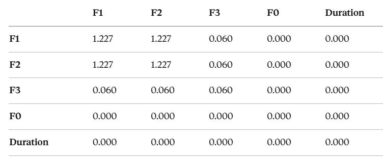
Heatmap of G matrix showing the dominant F1–F2 block and weak F3 coupling]

Three things jump out:

1. F1 and F2 are geometrically inseparable. G₁₁ = G₂₂ = G₁₂ = 1.227. The F1 and F2 rows are nearly identical — the tree always uses them together on every root-to-leaf path. They form a single geometric unit. This is exactly right: the F1–F2 plane is the primary vowel space in phonetics. The tree discovered this independently.

2. F3 has weak but non-zero coupling. G₃₃ = 0.060 with off-diagonals G₁₃ = G₂₃ = 0.060 to F1 and F2. F3 plays a supporting role — the tree uses it on some paths but not all.

3. F0 and Duration are geometrically dead. All zeros. The tree never splits on them. They contribute nothing to the geometry.

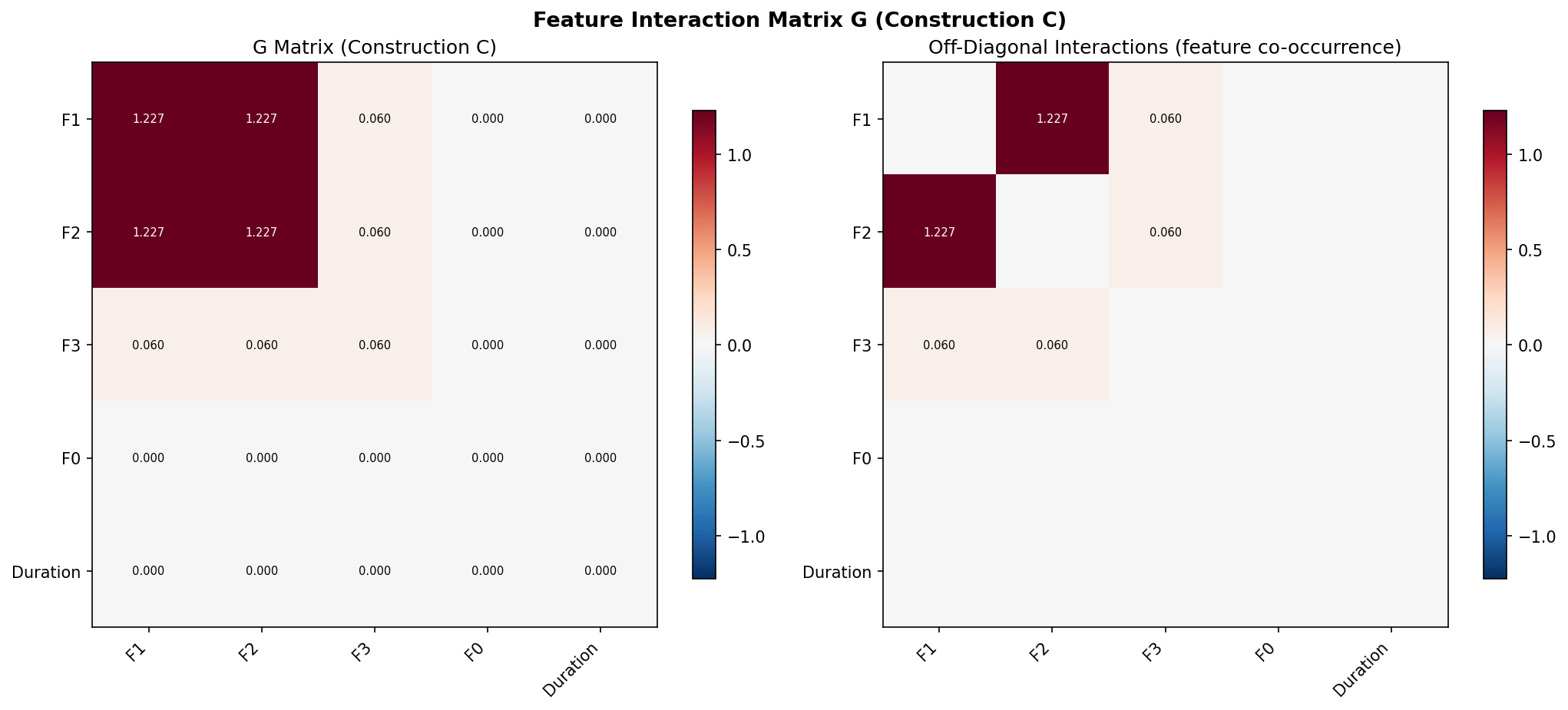
The eigenvalues of G are λ = [2.457, 0.057, 0, 0, 0] — a 43:1 ratio. The tree’s geometry is effectively one-dimensional, dominated by a single direction that combines F1 and F2.

Eigenvalue spectrum of S’ and per-feature geometric activity

---

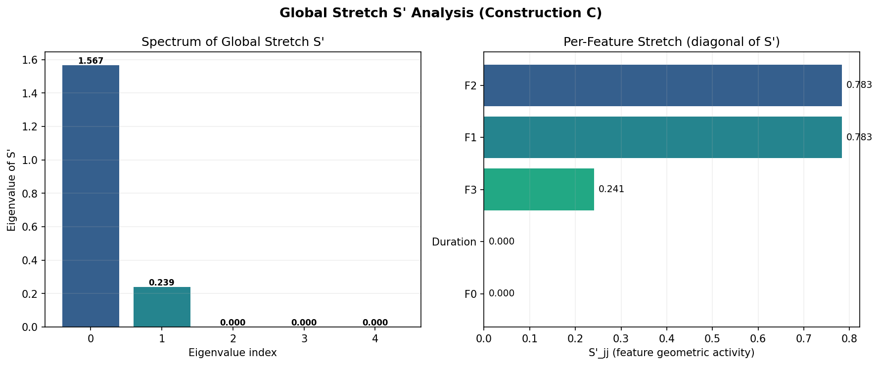
Feature loadings: what the eigenvectors tell us

The eigenvectors of G reveal how original features map to geometric principal components:

Feature loadings onto eigenvectors of S′

PC1 (λ = 1.567) loads equally on F1 and F2 at −0.71 each — this is the primary vowel space direction. PC2 (λ = 0.239) loads almost entirely on F3 (1.00) — capturing speaker-specific vocal tract resonance. PC3 through PC5 have zero eigenvalues; F0 and Duration each occupy their own dead eigenvector.

The tree’s geometry concentrates 87% of its spectral energy into a single direction that combines the two formant frequencies. This isn’t PCA — it’s not finding maximum variance. It’s finding the directions the tree actually uses for splitting.

---

The hidden feature: boundary vs. within-leaf importance

This is the most surprising result. Compare two notions of feature importance:

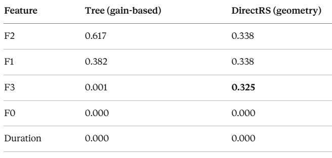
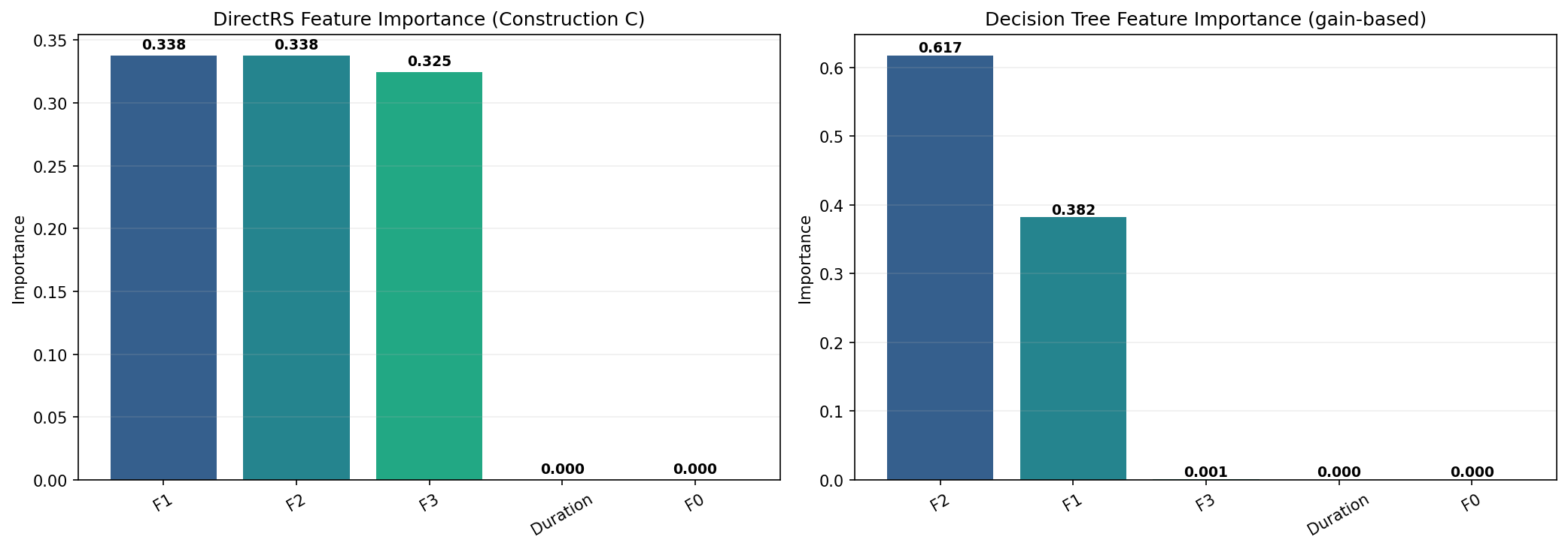
Side-by-side comparison of tree gain-based vs. DirectRS geometry-based importance]

The tree’s gain-based importance says: “F2 is king (62%), F1 helps (38%), everything else is irrelevant.”

DirectRS says: “F3 accounts for 32.5% of the local linear corrections — equal to F1 and F2.“

What’s happening? F1 and F2 define the partition boundaries — they decide which leaf you land in. But F3 varies systematically within leaves and is highly predictive of the residual classification error. The tree barely uses F3 for splitting (gain = 0.1%), but logistic regression discovers it’s critical for refining class probabilities given the partition.

This is a decomposition of importance into boundary importance (what carves the space) and within-leaf importance (what improves predictions inside each region). The standard tree never reveals the second kind. DirectRS does.

---

S’ embedding vs. PCA

The geometry-aware embedding z = S′x is fundamentally different from PCA:

S′ embedding vs. PCA: scatter plots and spectral concentration comparison]

PCA finds directions of maximum variance: V_PCA = 𝔼[xxᵀ]. The global stretch finds directions of maximum geometric activity: G = Σ w_ℓ A_ℓ. On the Hillenbrand data, Duration has substantial variance but zero geometric activity (the tree never splits on it), while F3 has lower variance but non-zero geometric activity. The S′ embedding concentrates 87% of its spectral energy in the first component vs. 67% for PCA — it’s more efficient because it focuses on predictively relevant directions rather than all variation.

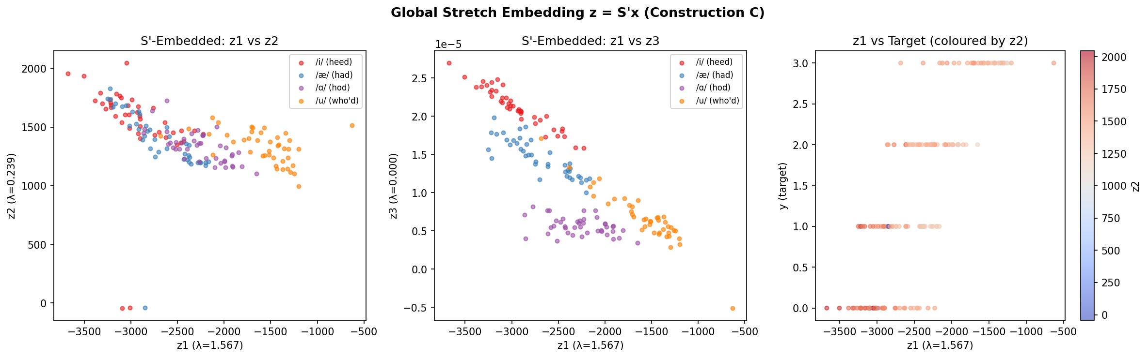
Global stretch embedding z = S′x colored by vowel class]

---

What this means

We started with an 8-leaf decision tree. By reading its path structure, we extracted a 5 × 5 stretch matrix that:

1. Revealed F1–F2 form an inseparable geometric unit (matching phonetic theory)

2. Exposed F3 as equally important for within-leaf corrections (invisible to gain-based importance)

3. Improved AUC from 0.986 to 0.989 and reduced Brier score by 37.8%

4. Connected tree ensembles to kernel methods and Gaussian processes

No gradient descent. No hyperparameter search (beyond logistic regression C). No black boxes.

The geometry was always there. We just needed to read it.

---

What’s next

This tutorial covered a single tree. The method extends naturally to ensembles:

\(G = \sum_{t=1}^T \sum_{\ell \in \text{leaves}(t)} w_{t,\ell} A_{t,\ell} \)

And there’s a deeper connection waiting: each leaf can be represented as a rotor in Clifford algebra Cl(d, 0) rather than a matrix — preserving orientation, enabling geodesic interpolation between leaves, and connecting tree ensembles to geometric algebra.

That’s the future post.

---

Full mathematical treatment with proofs: “Extracting Geometric Structure from Decision Trees” (Sudjianto & Zhang, 2026)

Code and data available for replication. Questions? Comments below.